Keypoints
Introduction
- Recommendation systems are one of the predominant systems in market like Netflix, amazon and Walmart.
- And also this applies to offline systems such as which product goes in which row to capture the users. And it is one of the challenging problems.
- The solution for that problem is called Collaborative Filtering.
Collaborative Filtering
- The Collaborative Filtering technique refers to looking at what products the current user has used or liked, find other users that have used or liked similar products, and then recommend other products that those users have used or liked.
- Lets looks at an example using a MovieLens dataset.
| |
- With this we can now handle the data with in the
ratingsdata frame. We can do an experiment to assign few scores to users and then get the average to multiply that with the movie score but we might end up with a match or not match. - This is entirely not right because in first place we need latent factors to know how to score the movies for each user.
Latent Factors
Latent factors allows us to learn how to score the products for each user set.
- Below are the steps:
Step 1: Randomly initialize some parameters. These parameters will be a set of latent factors for each user and movie. We will have to decide how many to use.
Step 2: Calculate the predictions. We can do this by simply taking the dot product of each movie with each user. The dot product will be very high for the ones that have a great match otherwise the product will be very low.
Step 3: Calculate the loss using any loss function.
- Now after this we can optimize our parameters (that is, the latent factors) using stochastic gradient descent, such as to minimize the loss or in other words the user movies recommendations.
- But some times due to the overfitting we can observe that the validation loss get worse and we can use a regularization technique like weight decay.
Weight Decay
- Weight decay also called as L2 regularization, consists of adding sum of all the weights squared to your loss function.
- When we compute the gradients, it will add a contribution to them that will encourage the weights to be as small as possible and this would prevent overfitting.
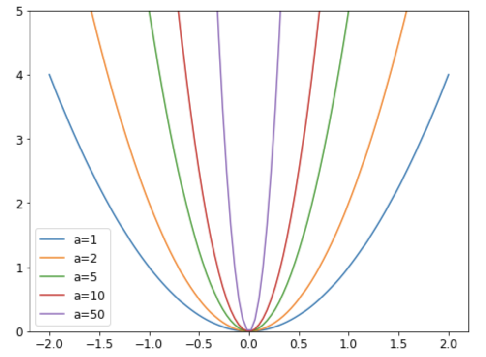
- For a simple function like parabola, we have the following graph.
- Limiting our weights from growing too much is going to complicate the training of the model, but it will yield a state where it generalizes better.
- To use the weight decay in fastai, just pass wd in your call to fit or fit_one_cycle. And this would yield better results.
| |
All the code is from the fastbook1
- We can create and train a collaborative filtering model using fastAI with below code:
| |
Bootstrapping
- The bootstrapping problem is a biggest challenge problem in collaborative filtering and refers to having no users to learn from.
- One solution would be to gather meta information from users like what genres would they like or what films they would choose from a selected few.
- One of the main problems in these cases would be the bias that would be introduced initially through the feedback loops.
- One of the approach that works better with this problem would be the Probabilistic Matrix Factorization/ (PMF) or we could apply deep learning to solve the issues related.
Deep Learning for Collaborative Filtering
- As a first step, we need to concatenate the results of embedding and activations together.
- This gives us a matrix which we can then pass through linear layers and nonlinearities in the usual way.
Step 1: Getting the embeddings
| |
Step 2: Creating a model with the embeddings
Step 3: Create a Learner and train the model
| |
Step 4: FastAI collab_learner function
| |
- The learn.model is an object of type EmbeddingNN.
Conclusion
- EmbeddingNN allow us to do something very important: we can now directly incorporate other user and movie information, date and time information, or any other information that may be relevant to the recommendation.
- We now have a brief understanding of how gradient descent can learn intrinsic factors or biases about items from a history of ratings which can provide some insights into the data.