Keypoints
Introduction
It is better to fail fast than very late. And it is always better to run more experiments on a smaller dataset rather running a single experiment on a large dataset.
- This chapter introduces a new dataset called Imagenette1
- Imagenette is a subset of the original Imagenet dataset but has only 10 categories of classes which are very different. This dataset has full-size, full-color images, which are photos of objects of different sizes, in different orientations, in different lighting, and so forth.
Imagenette
Important message: the dataset you get given is not necessarily the dataset you want.
- This dataset has been created by fast.ai team to quickly experiment with the ideas and to give the opportunity to iterate quickly.
- Lets see how can we work with this dataset and then apply techniques which can be used on larger datasets like Imagenet as well.
Step 1: Downloading dataset & building The Datablock
| |
Step 2: Creating a Baseline & Training the model
| |
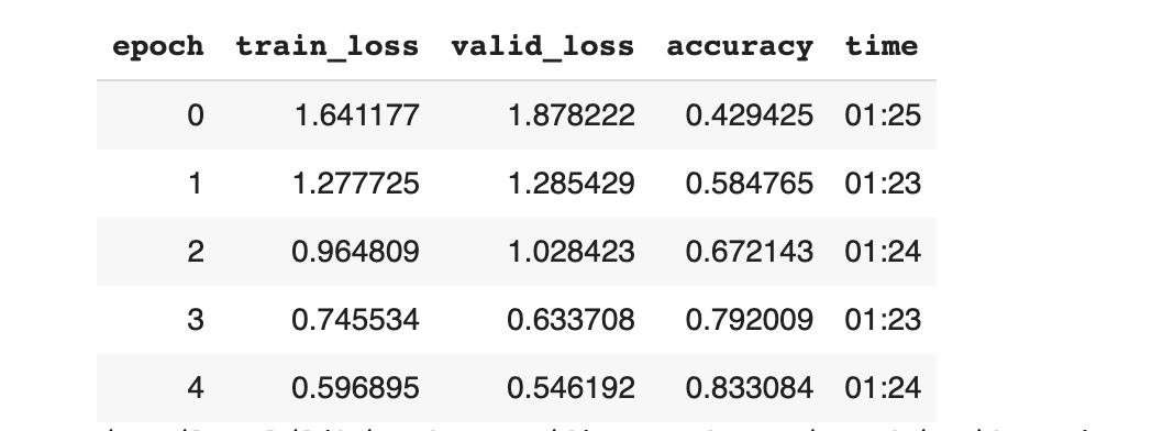 All the results are from my colab2
- So far we have achieved about 83.3% of accuracy. Let’s try to apply some techniques that would improve the performance.
Normalization
One of the strategy in the data pre-processing that will help a model perform better is to normalize the data.
- Data which has mean of 0 and a standard deviation of 1 is referred as Normalized data. But most of the data like images used is in between 0 to 255 pixels or between 0 & 1.
- So, we do not have the normalized data in either case. So to normalize the data, in fastAI we can pass Normalize transform.
- This transform will take the mean and standard deviation we want and transform the data accordingly.
- Normalization is an important technique that can be used when using pre-trained models.
Note: When using the cnn_learner with a pre-trained problem, we need not add the Normalize transform since the fastAI library automatically adds it.
Step 3: Adding Normalization
| |
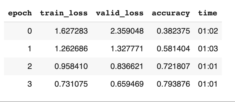
Step 4: Training the model again with normalization added
- After normalization, we have achieved an accuracy of 82.2%. Not an huge improvement from the previous, but for some strange reason there is a slight drop in performnace.

- The other technique we can employ here for training is ti start small and then increase as required.
- All the above steps are confined to train images which are at size 224. So, we can start with much smaller size and increase it and this technique is called Progressive Resizing.
Progressive Resizing
Progressive resizing: Gradually using larger and larger images as you train.
- Spending most of the epochs training with small images, helps training complete much faster.
- Completing training using large images makes the final accuracy much higher. In the process, since we will be using different size of images, we can use fine_tune to tune the model.
- And if we closely observed this is kind of a data augmentation technique.
Step 5: Create a data loader and try to fit into the model.
| |
Step 6: Replace the data loader and fine_tune it.
| |
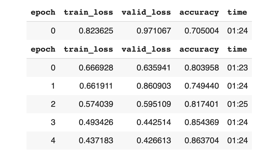
- From the above step it is evident that the Progressive resizing has achieved a good improvement in the accuracy of about 86.3%.
- However, it’s important to understand that the size of the Image at maximum could be the size of the image available on disk.
- Also, another caution on the resizing part is to not damage the pertained weights.
- This might happen if we have the the pre-trained weights similar to the weights in the transfer learning.
- The next technique to apply to the model is to apply data augmentation to the test set.
Test time Augmentation
Test Time Augmentation (TTA): During inference or validation, creating multiple versions of each image, using data augmentation, and then taking the average or maximum of the predictions for each augmented version of the image.
- Traditionally we use to perform training data augmentation with different techniques.
- When it comes to validation set, the fastAI for instance applies the center cropping.
- Center cropping is useful in some use cases but not all.
- This is because cropping from center may entirely discard any images on the borders. Instead on way would be to stretch and squish instead of cropping.
- However this becomes a hectic problem for model to learn those new patterns.
- Another way would be to select a number of areas to crop from the original rectangular image, pass each of them through our model, and take the maximum or average of the predictions.
- We could do this around different values across all of our test time augmentation parameters. This is known as /test time augmentation/ (TTA).
Step 7: Trying TTA
| |
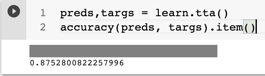
- We can see that the above technique has turned out well on improving accuracy to about 87.5%.
- However the above process slows down the inference by number of times we are averaging for TTA. So we can try another technique called Mixup.
Mixup
- Mixup is a very powerful data augmentation technique that can provide dramatically higher accuracy, especially when you don’t have much data and don’t have a pre-trained model that was trained on data similar to your dataset.
- Mixup technique talks about the data augmentation for the specific kind of dataset and fine tuned as needed.
Mixup works as follows, for each image:
- Picking a random image from your dataset.
- Picking a weight at random.
- Taking a weighted average (from step 2) of the selected image with your image; this will be your independent variable.
- Taking a weighted average (with the same weight) of this image’s labels with your image’s labels; this will be your dependent variable.
Note: For mixup, the targets need to be one-hot encoded.
- One of the reasons that Mixup is so exciting is that it can be applied to types of data other than photos.
- But, the issue with this technique might be the labels getting bigger than 0 or smaller than one as opposed to the one-hot encodings.
- So, we can handle this through label smoothing.
Label Smoothing
- In “Classification Problems”, our targets are one-hot encoded, which means we have the the model return either 0 or 1.
- Even a smallest of the difference like 0.999 will encourage the model to overfit and at inference the model that is not going to give meaningful probabilities.
- Instead to avoid this we could replace all our 1s with a number a bit less than 1, and our 0s by a number a bit more than 0, and then train. This is called label smoothing.
- And this will make the model generalize better.
Conclusion
- All the techniques described above are kind of eye opening on how we can build techniques that could augment each other and sometimes better than others.
- All these techniques will be applied to a real dataset and results will be published soon with description.