Keypoints
Lets recognize the Hand Written Digits via MNIST database.
- A image is an array of numbers / pixels under the hood.
- We need this because a computer only understand numbers.
- So, we try to convert all images into numbers and hold them in a data structure like Numpy Array or PyTorch tensor which will make the computations easier.
- Each Image is two dimensional in nature since they are grey scaled.
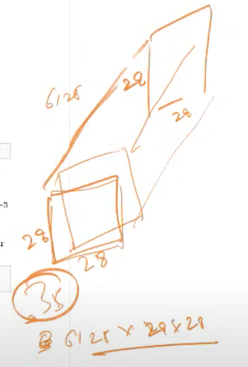
- All the images are now stacked to create a single tensor of 3 dimensions which will help to calculate the mean of each pixel.
- Now we do this mean calculation to achieve a single image of 3 or 7, which our model learns as an ideal 3 or 7.
- Now given an image of 3 or 7 whether from a training set or validation set we can use distance techniques like L1 norm or L2 norm to compute the distance between that image and the ideal 3 or 7 image.
- So the accuracy is the metric we will consider for knowing how good our model is performing.
Simple Example:
| |
- Both Numpy Array & PyTorch Tensor are same except for the naming. An Numpy array is a simple 2-dimensional representation of the image where as the PyTorch tensor is a multi-dimensional representation of the image. The below image shows the example of an image illustrated as an array & tensor and its dimensions.
Note: Since the image is a simple grey image (No Color), we have just 2 dimensions. If it’s an color image than we would have 3 dimensions (R,G,B).
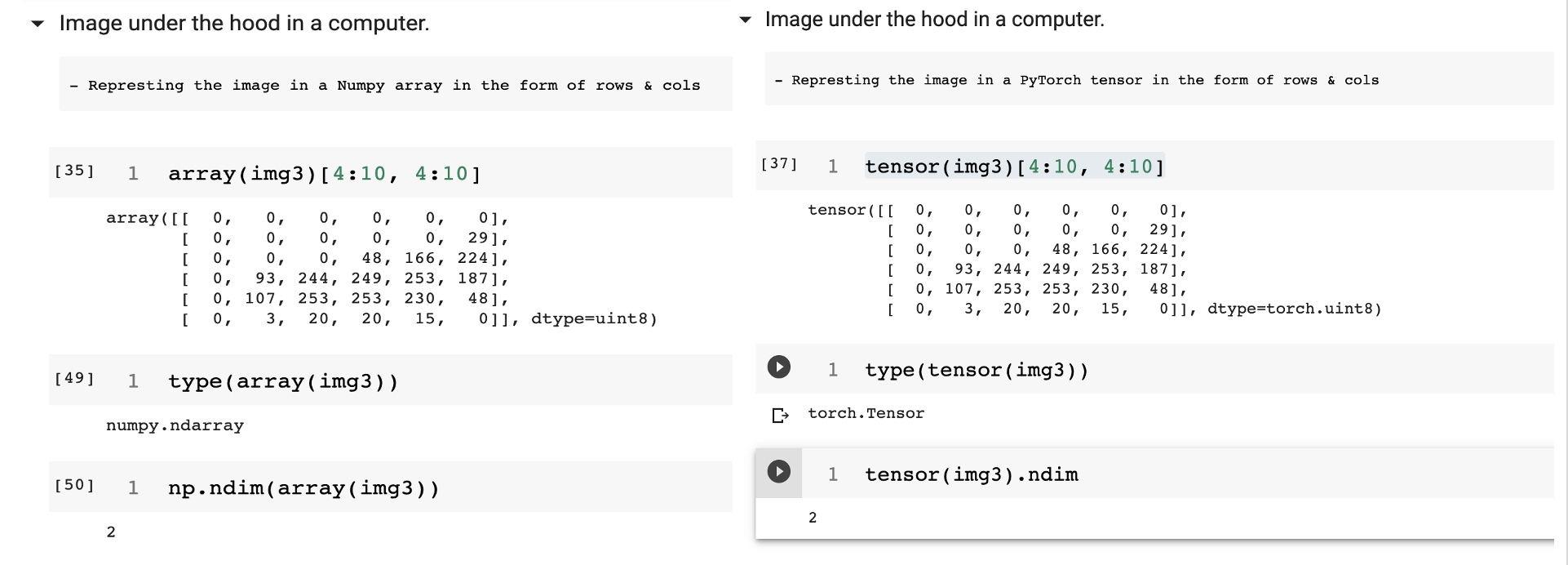
- Each number in the image array is called a Pixel & each pixel is in between 0 to 255.
- The MNIST images are 28 * 28 (total image size 784 pixels).
- A Baseline is a simple model which will perform reasonably well. So it is always better to start with a baseline and keep improving the model to see how the new ideas improve the model performance/accuracy.
- Rank of a Tensor: A Rank of a tensor is simply the number of dimensions or axes. For instance, a three dimensional tensor can also be referred as rank-3 tensor.
- Shape of Tensor: Shape is the size of each axis of the tensor.
- To get an ideal image of 3 or 7, we need to perform the below steps: (Each Function shown here is explained in detailed with examples in the next section).
- Convert all the images into tensors using
tensor(Image.open(each_image)). - Wrap the converted images into a list of image tensor’s.
- Stack all the list of image tensors so that it creates a single tensor of rank-3 using torch.stack(list_of_image_tensors). In simple terms a 3-dimensional tensor.
- If needed we have to cast all of the values to float for calculating mean by using float() function from pytorch library.
- Final step is to take the mean of the image tensors along dimension-0 for the above stacked rank-3 tensor using mean() function. For every pixel position, the mean() will compute the average of that pixel over all the images.
- The result, is the tensor of an ideal 3 or 7 calculated by computing the mean of all the images which will have 2-dimensions like our original images.
- To classify if an Image is a 3 or 7, we can use a simple technique like finding the distance of that image from an ideal 3 or ideal 7 computed in the earlier steps.
- Distance calculation can be done using either L1 normalization or L2 normalization. A simple distance measure like adding up differences between the pixels would not yield accurate results due to positive & negative values (Note: Why Negative Values ? Remember we have lot of 0’s in the image and other image may contain a value at that same pixel which would result in a negative value).
- L1 norm: Taking the mean of the absolute value of the differences between 2 image tensors. A absolute value abs() is a function that replaces negative values with positive values. This is also referred as Mean Absolute difference. This can be calculated using
F.l1_loss(any_3.float(), ideal_3). - L2 norm: Taking the mean of the square of the differences and then take a square root. So Squaring a difference will make the value positive & then square root cancels the square effect. This is also referred to as Root Mean Squared Error (RMSE). This can be calculated using
F.mse_loss(any_3.float(), ideal_3). - The result of the above computation would yield the loss. Higher the loss, lesser the confidence of that image being 3 vs 7.
- In practice, we use accuracy as the metric for our classification models. It is computed over the training data to make sure overfitting occurs.
- Broadcasting is a technique which will automatically expand the tensor with the smaller rank to have same sizes as one with the larger rank.
| |
- In broadcasting technique the PyTorch never creates copies of lower ranked tensor.
Some of the new things learned from fastAI library:
- ls() → L - A function that list the count of items & contents of the directory. It returns a fastai class called L which is similar to python built-in List class with additional features.
- Image.open() → PngImageFile: A class from Python Image Library (PIL) used for operations on images like viewing, opening & manipulation.
| |
- A Pandas.DataFrame(image) → DataFrame: A function that takes an image, converts that into a DataFrame Object & returns it.
- We can set some style properties on a dataframe to see the color coding and understand it better.
| |
- np.array(img) → Numpy.Array: Numpy’s array function will take an image and return the pixels of the image in a two dimensional data structure called Array.
- tensor(img) → PyTorch.Tensor: PyTorch’s tensor function will take an image and return the pixels of the image in a multi-dimensional data structure called Tensor.
- List Comprehensions in python returns each value in the given list based on a optional condition when passed to any function f().
| |
- show_image(tensor) → Image: A fastai function which takes an image tensor & display the image.
- torch.stack(list_of_tensors) → PyTorch.Tensor: A Pytorch function that takes a list of tensors (2-dim image tensors) and create a 3-dimensional single tensor (rank-3 tensor). This will be useful to compute the average across all the images.
torch.tensor.float() → float_value: Casting the values from int to float in PyTorch gives the ability to calculate the mean.
- L1 norm can be performed using the following
1 2 3dist_3_abs = (any_image_of_3 - ideal_3).abs().mean() # Note: ideal_3 is the 3 calculated by compuitng mean of the stacked rank-3 tensor.- L2 norm can be performed using the following
1dist_3_sqr = ((any_image_of_3 - ideal_3)**2).mean().sqrt()- The above distances can be also computed using the inbuilt PyTorch lib functions from torch.nn.functional package which is by default imported as F by fastai as recommended.
1 2 3 4 5# L1 norm: F.l1_loss(any_3.float(),mean7) # L2 norm: F.mse_loss(any_3,mean7).sqrt()Stochastic Gradient Descent is the way of automatically updating the weights of the neural network input’s, based on the previous result to gain the maximum performance or in simple terms better accuracy.
This can be made entirely automated, so that the network can reach back to the initial inputs, update their weights and can perform the training again with the new weights. This process is called the back-propagation.
Example of an function that can be used to classify a number based on the above described way:
| |
- In the above function, x - vector representation of the input Image. w - vector of weights
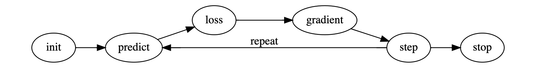
How can we make this function into a Machine Learning Classifier:
- Initialize the weights.
- For each image use these weights to predict whether a 3 or a 7.
- Calculate the loss for this model based on these predictions.
- Calculate the gradient, which helps to determine the change in the weight and in turn the loss for that weight. And this has to be done for each weight.
- Change the weights based on the above gradient calculation. This step is called “Step”.
- Now we need to repeat from prediction step (step 2). Iterate until your model is good enough.
Detailing the each step in the above process:
- Initialize: Initializing the parameters/ Weights to random values will perfectly work.
- Loss: We need a function that return the loss in terms of a number. A good model has small loss and vice versa.
- Step: We need to determine whether to increase the weights or decrease the weights to maximize the performance or in other terms minimize loss. Once we determine the increase or decrease then we can increment/decrement accordingly in small amounts and check at which point we are achieving the maximum performance. This process is manual and slower and can be automated and achieved by calculating gradient using calculus. Gradient calculation will figure out directly whether to increment / decrement weights and by how much amount.
- Stop: This is where we will decide & implement about number of epochs to train our model . In the case of digit classifier, we will train our model until over fitting (Our model performance gets worse) occurs.
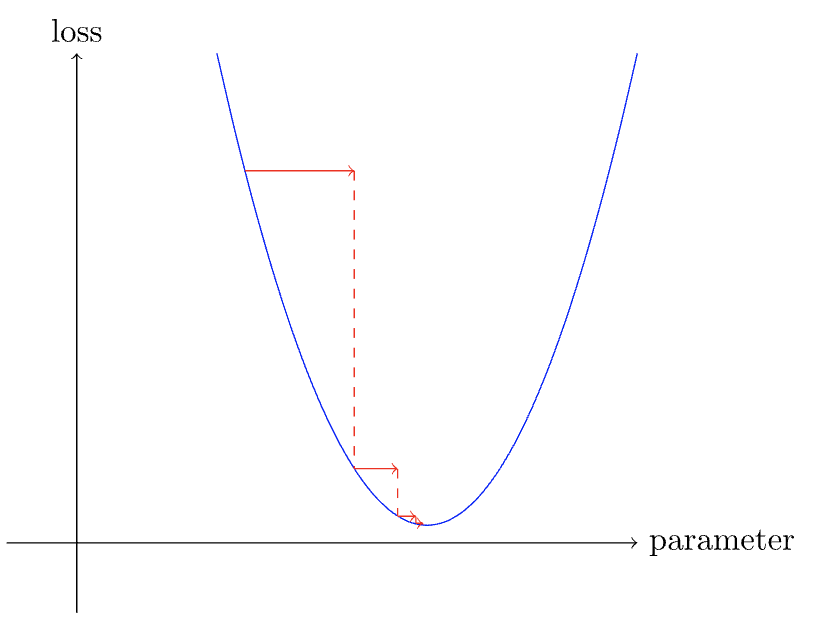
Example of a simple loss function and understand about slope
| |
- Visualizing the above function with slope at one point , when initialized it with a random weight parameter.
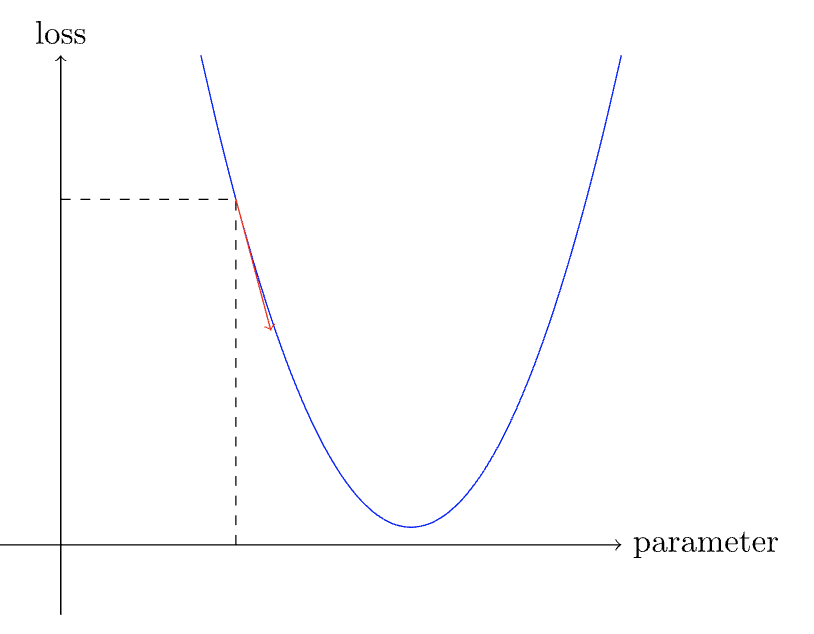
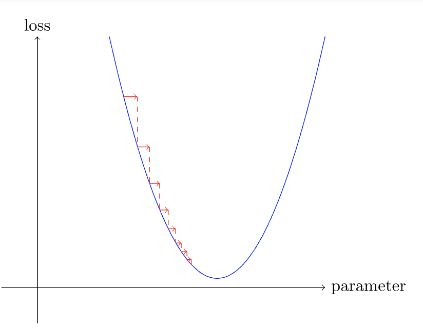
- Once we determine the direction of the slope, then we can keep adjusting the weight, calculate the loss every time and repeat the process until we reach the lowest point on the curve where the loss is minimum.
- For gradient calculation, reason behind using calculus over doing it manually is to achieve performance optimization.
Calculating Gradients, Derivatives & why do we need them: What & Why:
- In simple words, gradient will tell us how much each weight has to be changed to make our model better. And it is a vector and it points in the direction of steepest ascent to minimize the loss.
- A derivate of a function is a number which tells us, how much a change in parameter will change the result of the function.
- For any quadratic function, we can calculate its derivative.
- Important Note: A derivative is also a function, which calculates the change, rather than a value like a normal function does.
- So, we need to calculate gradient to know how the function will change with a given value so that we can try to reduce the function to the smallest number where the loss is minimum.
- And the computational shortcut provided by calculus to do the gradient calculation is called Derivative.
How to we calculate derivates:
- We need to calculate gradient for every weight since we don’t have just one weight.
- We will calculate the derivative of one weight considering the others as constants and then repeat the process for every other weight.
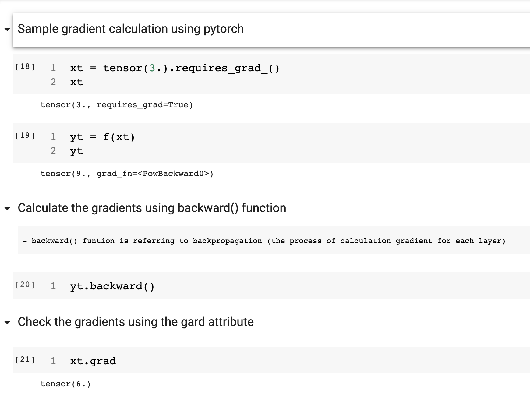
- A pytorch example to calculate derivative at value 3
| |
- In deep learning, the “gradients” usually means the value of a function’s derivative at a particular argument value.
Example of a gradient calculation: Consider we want to calculate derivative of x*2 and the result is 2x, where x=3, so the gradient must be 2 x 3 = 6
- The gradient only tell us the slope of the functions and not exactly how much weight we have to adjust. But the intuition is if we have a big slope then we need to make lot of adjustments to weights and vice versa if the slope is small then we are almost close to optimal value.
How do we change Weights/Parameters based on Gradient Value:
- The most important part of the deep learning process is to decide how to change the parameters based on the gradient value.
- Simplest approach is to multiply the gradient with a small number often between 0.001 and 0.1 (but not limited to this range) and this is called Learning Rate(LR).
- Once we have a Learning Rate we can adjust our parameters using the below function
- This process is called as stepping the parameters using the Optimizer step. This is because, in this step we are trying to find an optimal weight.
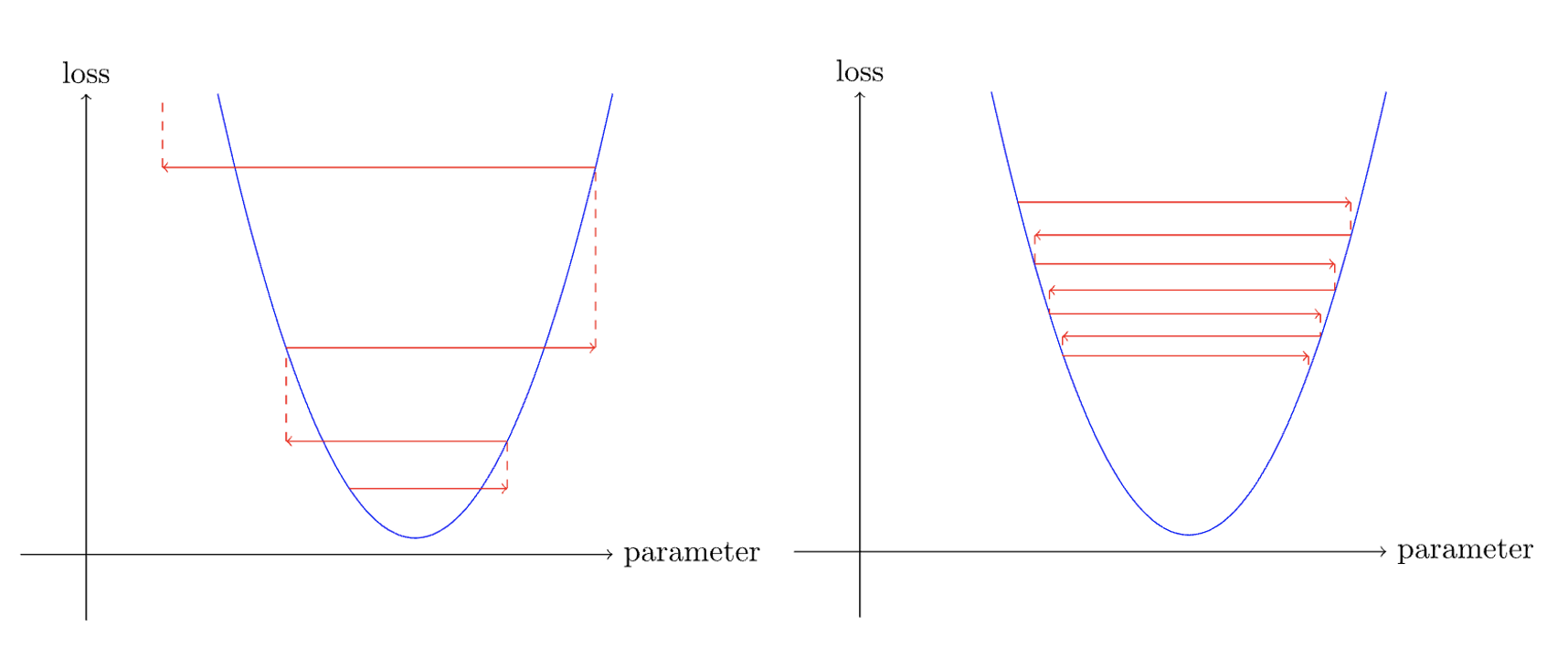
- We can pick either very low learning rate or a very high learning rate and both have their consequences.
- If we have a low learning rate then we have to do lot of steps to get the optimal weight.
- Picking a very high learning rate is even worse and can result in the loss getting worse(left image) or may bounce around(right image, requiring lot of steps to settle down) . So we are loosing our goal of minimizing the loss.
Conclusion:
- We are trying to find the minimum (loss) using the SGD and this minimum can be used to train a model to fit the data better for our task.
Some miscellaneous Key-points:
- All Machine learning datasets follow a common layout having separate folders for training and validation (test) set’s.
- A Numpy array & a PyTorch tensor are both multi-dimensional arrays and have similar capabilities except that the Numpy doesn’t have GPU support where as PyTorch does.
- PyTorch can automatically calculate derivates where as Numpy will not which is a very useful feature in terms of deeplearning.